Positional Encoding from Sinusoidal to RoPE

Transformers process the tokens of a text input in parallel, but unlike sequential models they do not understand position and see the input as a set of tokens. However, when we calculate attention for a sentence, words that are the same but in different positions do receive different attention scores. If attention is a calculation between two embeddings, how can the same word, i.e., same embedding, receive different scores when it is in a different position? It comes down to positional encoding, but before we get into how positional encoding works, let’s run a test.

import torch
import torch.nn as nn
from transformers import AutoTokenizer, AutoModel
import matplotlib.pyplot as plt
import seaborn as sns

model_name = "bert-base-uncased"

# define sentence
sentence = "The brown dog chased the black dog"

#define tokenizer
tokenizer = AutoTokenizer.from_pretrained(model_name)
tokens = tokenizer(sentence, return_tensors="pt")["input_ids"]

# define token embeddings
model = AutoModel.from_pretrained(model_name)
token_embeddings = model.get_input_embeddings()(tokens)
embed_dim = token_embeddings.shape[-1]

class SimpleAttention(nn.Module):
    def __init__(self, embed_dim):
        super().__init__()
        self.w_query = nn.Linear(embed_dim, embed_dim)
        self.w_key = nn.Linear(embed_dim, embed_dim)
        self.w_value = nn.Linear(embed_dim, embed_dim)

        # Initialize weights
        nn.init.normal_(self.w_query.weight, mean=0.0, std=0.8)
        nn.init.normal_(self.w_key.weight, mean=0.0, std=0.8)
        nn.init.normal_(self.w_value.weight, mean=0.0, std=0.8)

        self.attention = nn.MultiheadAttention(embed_dim=embed_dim, num_heads=1, batch_first=True)

    def forward(self, x):
        output, attention_weights = self.attention(self.w_query(x), self.w_key(x), self.w_value(x))
        return output, attention_weights
    
# Compute attention        
attention_layer = SimpleAttention(embed_dim=embed_dim)
attention_output, attention_weights = attention_layer(token_embeddings)

# Convert attention weights to numpy array and remove extra dimensions
attention_matrix = attention_weights.squeeze().detach().numpy()

# Get token labels for the axes
tokens_text = tokenizer.convert_ids_to_tokens(tokens[0])

# Create heatmap
plt.figure(figsize=(10, 8))
sns.heatmap(attention_matrix, 
            xticklabels=tokens_text,
            yticklabels=tokens_text,
            cmap='YlOrRd',
            annot=True,
            fmt='.2f')

plt.title('Attention Weights Heatmap')
plt.xlabel('Key Tokens')
plt.ylabel('Query Tokens')
plt.tight_layout()
plt.show()

The code above will create a simple attention layer, without positional encoding. This enables our test to demonstrate how attention behaves when all tokens are treated purely based on their semantic embedding, without any positional differentiation. It has been initialized with random weights and has not undergone training; however, training shouldn’t matter as tokens that are the same will have the same weights applied to them and result in the same output.

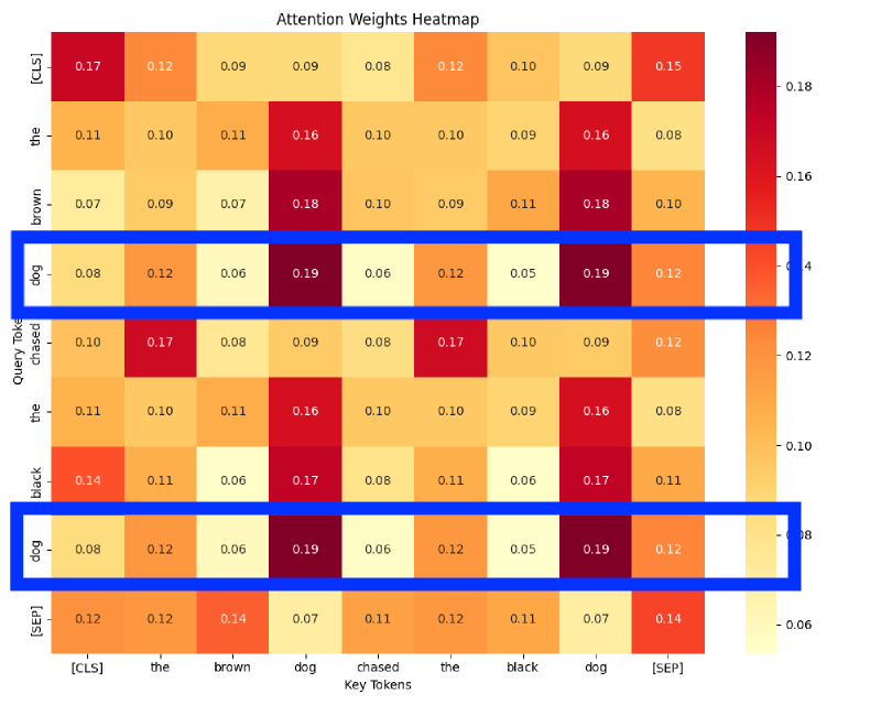
The attention heat map above is the output of our code. I’ve highlighted the use of two dog tokens to demonstrate how they receive equivalent attention weights against all other keys. For attention heads to be able to specialize, e.g., notice verb-object pairs, they must be able to differentiate between the same words in different positions, otherwise they will receive the same result from the same weights being applied to token embedding.

What do positional encodings enable

#

In transformers we differentiate words at different positions with positional embeddings. This transformation perturbs the embedding based on the position of the word. For our example sentence in the code above, dog at position 3 would have a slightly different embedding to dog at position 7 after positional embeddings have been applied, resulting in a different attention result for each token. This allows attention heads to see different positions and specialize. For example, an attention head that specializes in recognizing verb-object pairs would have high attention with chases and the second dog, but not the first dog. Without the slight alteration to each dog’s embedding, that specialized attention head could never notice the difference between the two.

Positional encodings step by step

#

Before we start to think about how positional encodings might be implemented, let’s come up with some requirements

This is instead of passing in an additional feature, which would mean our neural network has to interpret extra information and spend extra computation. By combining with the existing embedding, we need a way for the network to see a different embedding when words are the same at different positions.

As shown earlier, each word needs to be uniquely identified even if the same word appears in a text sequence.

We want to create models that can generalize, therefore our positional encoding should be a pattern that can be recognized and accounted for in our attention matrices. We could assign random IDs to each position. In theory this is learnable, but we would be using more parameters than needed, since the network would have to memorize each ID alongside the semantic information it encodes. We are essentially forcing the transformer to memorize combinations of position and semantic information rather than allowing it to learn reusable patterns.

Add the position as an integer

#

An obvious thing to try is to simply add the position of the token to the embedding. For example, if dog was my first word and the embedding was [0.10, 0.80, 0.45], adding 1 to this would result in [1.10, 1.80, 1.45]. For the second word we would add 2 and so on.

There are a few problems with this. First, I could have many words in my input, and say I reach the 100th word. Adding 100 to each dimension of that token’s embedding will create very large numbers. In neural networks we want to keep inputs on a similar scale to allow for faster convergence, but with our implementation embedding values will grow as we add more words to our input.

This requirement will ensure that embeddings stay within reasonable limits and do not grow too large. Another problem presented by our larger integers is that the network will only be trained on the largest length it has seen, and therefore cannot generalize to any length. Ideally we want our network to work at lengths it has not seen.

Lastly, the positional part of our embedding seems to greatly outweigh the original embedding. It might be hard to see what the original input was; in fact, it seems to completely change the embedding and more strongly represent position than semantic information.

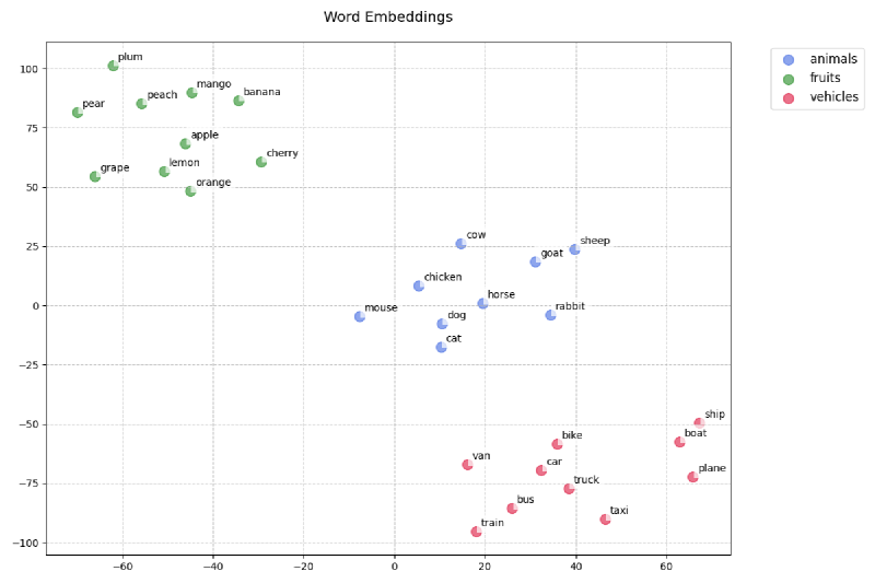
The graph above shows the embeddings of a random list of words without positional information in reduced dimensional space. We can see clear semantic meaning, with words around the same concept clustering together.

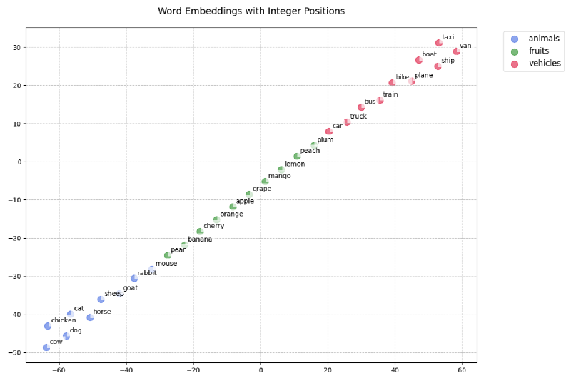
The graph above represents the same embeddings with integer positions added based on the position they were in the text sequence. We can see they no longer cluster as before and they seem to have a different semantic meaning. They also seem to be dominated by some increasing order. Therefore adding a position with an integer is probably not going to work for us and has led us to a new requirement.

Sinusoidal Encoding

#

Based on our requirements so far, we’ve now come to the solution presented in the Attention Is All You Need paper. Before jumping to it, let’s build up our understanding of how it works.

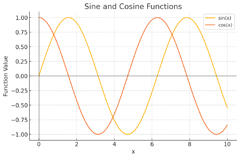
To help meet our requirements, let’s use a sine function, where the positional coding is sine(x), with x being our token position and the result added to our embedding element wise.

For example, if our embedding was [0.1, 0.6, 0.8] our resulting embedding with positional information would be [0.1 + sin(0), 0.6 + sin(1), 0.8 + sin(2)].

If we take the x axis to be our token position, we can see that the numbers produced are small, helping to retain our embedding semantic information if added to each embedding element wise. Requirement wise, it almost meets what we want: it can handle any sequence length as sine can be calculated for any x value, it is bounded between 1 and -1, and it isn’t large enough to alter semantic information. The one gap is requirement 2: Positional Encodings must uniquely identify every word in a sequence.

As we can see, sin(x) is periodic and it will eventually repeat itself for a token’s position. For example, sin(2) and sin(353) when rounded up will return the same value. This means for positions that return the same value, our attention mechanism will see them as the same position, and if they are the same word, we will have the same problem as not having positional encoding.

To help mitigate this we introduce cosine, i.e., cos(x) as shown above, and for each even index of our embedding we use sine and for odd indices we use cosine.

For example, if our embedding was [0.1, 0.6, 0.8] our resulting embedding with positional information would be [0.1 + sin(0), 0.6 + cos(1), 0.8 + sin(2)].

Using cosine introduces a phase shift and greatly reduces the likelihood of receiving the same value for a position later in the sequence, and the phase shift greatly reduces the chance of values being near each other. Even so, there is still a chance of repeating at longer sequence lengths, plus with the regular periodicity it is hard to build relative patterns across long distances. This means we might not be meeting requirement 3: We must be able to generalize over positional encoding patterns. With this shortwave frequency it will be hard to generalize long distance patterns.

We can improve on generalizing over long range patterns and reduce the chance of results collapsing into the same position by introducing lower frequencies. That is, we can create a general function which is sin(x/i) for even positions and cos(x/i) for odd positions, where i is the index of our embedding.

For example, if our embedding was [0.1, 0.6, 0.8, 0.9] our resulting embedding with positional information would be [0.1 + sin(1), 0.6 + cos(1/2), 0.8 + sin(2/3), 0.9 + cos(2/4)].

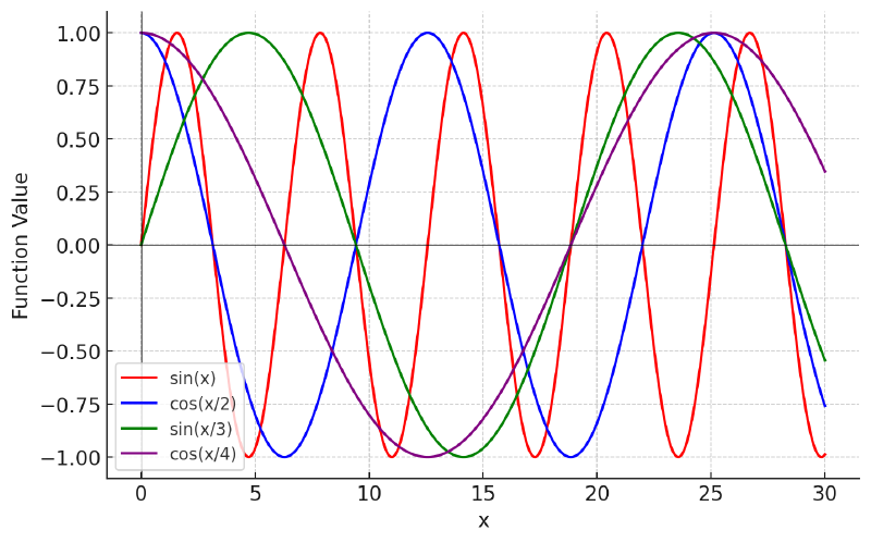
The graph has been expanded on the x axis compared to previous graphs, to show how dividing by the i-th position decreases the frequency. We would do this for all the dimensions of the embedding, therefore if our embedding size was 768, we would have 768 individual values, where the frequency decreases as we move closer to the end of the embedding.

The decreased frequency can be used to generalize over long distances, and the extra dimensions that highlight short, medium, and long distances allow our attention matrices to learn parameters that discard certain ranges and focus on what is needed for a particular attention head.

With our current solution, as we are only scaling up each embedding index linearly by increasing i, we could have many dimensions that don’t convey enough different information and therefore have redundant positional information.

Our current formulas are:

Above PE represents our positional encoding function, pos the token we are taking in, and i our embedding index.

In the Attention Is All You Need paper, the formulas used are

Here we can see that rather than dividing by i, we have i as an exponent of 10000 and i is divided by d, which represents the embedding size. This allows the different dimensions to scale up logarithmically, covering a wider range of frequencies rather than the previous linear scaling, and also reduces redundant positional information. Using 10,000 as the base with an exponent is what allows the frequencies to scale up logarithmically, and d is used to control the scaling. Without d, it would scale far too quickly and might mean we miss important positional information. 10,000 was used as the base after experimenting in the Attention paper and provided a balance between scaling up and capturing enough information at different ranges. This greater range of frequencies allows the model to generalize better, and gives more options for attention heads to focus on ranges for their specialization.

Absolute vs Relative Positional Encoding

#

So we’ve built out positional encoding in the same way that was designed in the Attention Is All You Need paper and this method has been used in many models. It has since been improved upon and subsequently used in newer transformer models.

The problem with sinusoidal encoding is that it falls into a category known as absolute positional encoding. Absolute encoding adds a particular value or ID to each position, so position 1 receives a certain value, position 2 another, etc. If I have the sentences “A man threw a ball” and another sentence “In the garden a man threw a ball”, in each sentence I have “man threw” in position 2, 3 and in position 5, 6 respectively. With sinusoidal encoding, man and threw will receive different positional encodings in each sentence. In language, though, what creates meaning is less about absolute positions of related words and more about the relative position between them. An attention head specialized in detecting subject and verb would have to learn the value for man and threw differently for the two sentences. By providing absolute values for each position, our learned parameters have less chance to generalize. There is some implicit relative positioning in sinusoidal encoding, from the periodicity of sine and cosine waves, but it’s hard to extract, and models are not forced to look at it when absolute positioning is available.

With relative positioning, if we took the same sentence our encoding scheme would receive values that highlight the relative position between words, rather than absolute values. This forces the model to use relative values and also helps it generalize more, a property we want for our NLP models. For example, in the case with man and threw in two sentences, our model could extract the fact that the words are next to each other, without having to memorize exact embedding plus positional values for different situations.

RoPE (Rotary Positional Embedding)

#

One way that has been used in many models to provide relative positional embeddings is RoPE.

Let’s imagine we have sentence 1 “The mouse ate some cheese” and sentence 2 “In the house a cat ate some cheese”

The graphs on the top represent simple 2D embeddings for each word in our sentences. The graph below represents a rotation of each vector based on their position using the transformation pθ, where p is the word position and θ is 25°. For example, some in the first sentence at position 4 would be rotated by 4θ, which is 100°. In the rotated embeddings, ate and cheese have the same relative position in each sentence. They end up at different absolute positions, but the angle between them is the same, because the relative distance between them is the same in each sentence. This is what RoPE does: it takes an embedding and rotates it by some θ based on its position.

RoPE and Attention Math

#

You can also see that every embedding has its magnitude maintained. No matter where we rotate, the magnitude will be the same. We can see the importance of this by looking at how we calculate attention scores.

We can see our attention scores rely on the norms of our vectors and the angle between them. Since we have only rotated our vectors, their norms stay the same, therefore any influence on attention scores due to RoPE must be on angle changes. Including the RoPE angle difference, our attention score now becomes the following, where d is the angle introduced by RoPE.

This means that if our attention head wants q and k to be highly aligned but they are far apart, the model has to compensate. It can learn to increase the magnitude of the original embedding when projected into q and k, or project them into a space where they are much closer despite RoPE moving them far apart.

We’ve seen how rotating embeddings helps transformers identify tokens at different positions by providing another lever to modulate: the angle between tokens. To see how relative position can be picked up by the model, we need to break down our attention score using transposition.

The above formula defines a RoPE transformation, where the first parameter is our vector, the second is the position in a text sequence, and R is a rotation matrix. Therefore our attention score would be:

Changing this to matrices transposition, and using product transposition rules.

Since R is a rotation matrix, and the transpose of a rotation matrix can be represented as R(-θ) we can simplify to

Where j and i are simply positions, we can see how the attention calculation has cleanly extracted the difference in positions, allowing it to use relative distance rather than being intertwined with the actual semantic content of the embeddings. This allows the model to modulate what it wants, such as direction or angle, to achieve the result we want. Before, with sinusoidal, we had to learn to extract position from the semantic information.

RoPE frequencies

#

As with the sinusoidal method previously talked about, you might be wondering if the rotation eventually repeats, making the same token at different positions appear at the same angle relative to another token. Like the sinusoidal method, RoPE introduces different frequencies across the embedding. In our example so far we have only considered 2D embeddings. In RoPE, within one embedding we take indices pairwise (e.g., positions 1 & 2, positions 3 & 4, etc.). Each pair is rotated by some θ, depending on the token position and the index of the pair. As we move further along the embedding, the rotation becomes smaller, resulting in a lower frequency towards the end, as in the sinusoidal method. This gives us unique signatures for repeated tokens in long text sequences. It also gives the model the data to focus on what it wants, such as long range or short range dependencies.

To rotate each pair we can use a rotation matrix

m is our token position and i-th θ is defined as

This is similar to our sinusoidal formula and produces similar sinusoidal frequencies, i being the pairwise position, and i-th θ is a rotation angle defined for each pair in an embedding based on its index.

For example, if our embedding was [0.1, 0.4, 0.5, 0.2], after splitting into pairs we have [[0.1, 0.4], [0.5, 0.2]]; our 1st pair is [0.1, 0.4] and 2nd pair [0.5, 0.2]. We then calculate theta for the 1st and 2nd pair using 1 and 2 as i.

Using the above sparse matrix we can rotate each pair of the embedding. We calculate θ up to d/2 because we use pairs and only need to compute angles for half the size of the embedding.

Efficient Implementation of RoPE

#

The sparse matrix can get quite large, and holding that in memory along with accompanying matrix multiply can be made more efficient by splitting up our rotation matrices into two vectors.

If we have a 2 dimensional embedding at position 1 rotating this would involve the calculation

We can break this down into the following components

First we use element wise multiplication to cover the cos part of our rotation matrix. Notice how we have left -x2 *sin(θ) on the top row and, x1 *sin(θ) on the bottom. As negative x2 is now on the top, for every pair we flip them and make x2 negative.

We then simply add the two results together element wise to achieve the same as sparse matrix rotation, but with a method that doesn’t require construction of large matrices and is more easily vectorized.

Sources & Further Reading

#

• You could have designed state of the art Positional Encoding – This post was heavily inspired by this original blog post.
• RoFormer: Enhanced Transformer with Rotary Position Embedding – Introduces RoPE (Rotary Positional Embedding), a technique for modeling relative positions through rotation.
• Attention Is All You Need – The original Transformer paper that introduced sinusoidal positional encodings and the self-attention mechanism.